Choosing the wrong Excel formula can produce a plausible but incorrect result. Start by defining what a row represents, checking missing values and deciding which question you need to answer. The functions and summary tools below are useful for small, structured datasets when their inputs and limitations are clear.
Excel includes many analysis functions, but useful work often starts with a few familiar operations. This guide keeps four functions, PivotTables and Quick Analysis in view. When the spreadsheet contains research observations, follow a research analysis process as well: a calculation does not establish why a person encountered a problem.
Useful Data Analysis Functions in Excel
1. CONCATENATE Function
CONCATENATE joins text values from several cells into one string. For example, =CONCATENATE(A2,"-",B2) combines an issue ID and category with a hyphen. It remains available for compatibility; current Excel also offers CONCAT and TEXTJOIN. Joining values does not validate an identifier, and dates or numbers may need explicit formatting to retain the representation you intend.

2. LEN Function
LEN returns the number of characters in a text string, including spaces. For example, =LEN(A2) returns 3 when A2 contains I01. This can flag unexpected lengths in an identifier column, but matching lengths do not prove that identifiers are valid or unique. Inspect the content and duplicates separately.
3. COUNTA Function
COUNTA counts cells that are not empty; it is not a test that each record is complete. Microsoft’s COUNTA documentation notes that empty text returned by a formula is counted. For example, =COUNTA(A2:A7) counts six populated issue IDs in the example below. A truly empty cell is different from a formula returning "" or a cell containing a space.
4. AVERAGEIFS Function
AVERAGEIFS returns the average of values that meet one or more criteria. Its syntax begins with the average range: =AVERAGEIFS(average_range,criteria_range1,criteria1,...). In the example, =AVERAGEIFS(C2:C7,B2:B7,"Navigation") averages 12, 18 and 15, returning 15 minutes. Use equally sized ranges and check the selected subset. Microsoft’s AVERAGEIFS reference explains its conditions and error cases.
The following six rows are illustrative issue-review data, not measured user results. Place the headers in A1:C1 and the rows in A2:C7 to reproduce the formulas. Minutes means time spent reviewing an issue; it does not measure user task completion or design effectiveness.
| Issue ID | Category | Minutes |
|---|---|---|
| I01 | Navigation | 12 |
| I02 | Labeling | 8 |
| I03 | Navigation | 18 |
| I04 | Empty states | 10 |
| I05 | Labeling | 6 |
| I06 | Navigation | 15 |

How to Do Data Analysis Using Excel
A PivotTable summarizes structured records by categories, using calculations such as count, sum or average. It helps inspect a dataset without manually rearranging the source rows. First decide what you want to compare and verify the data types; a numerical column stored as text can produce an unexpected summary. Microsoft’s PivotTable instructions cover supported versions and setup.
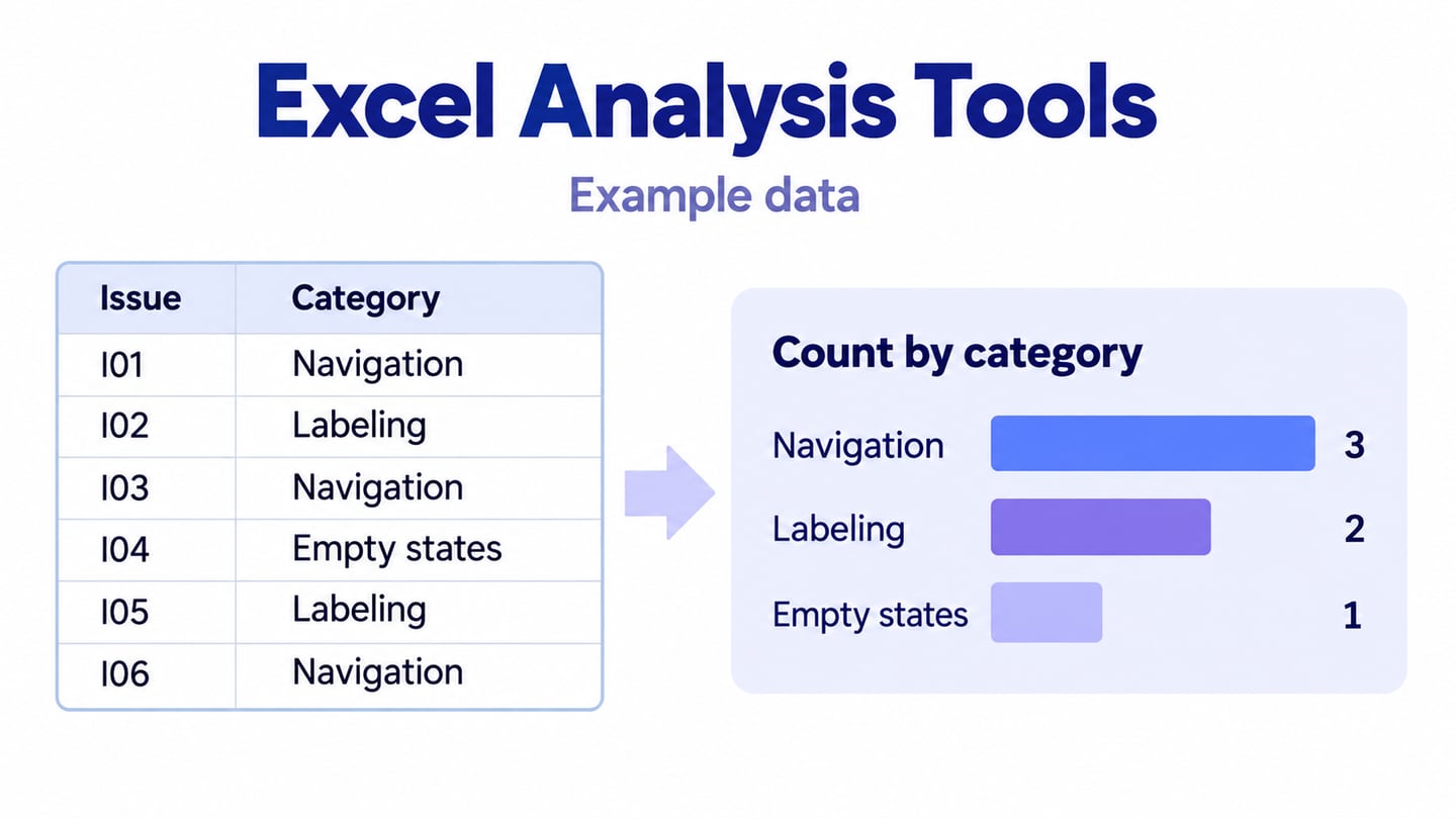
For the sample issue log, use Category as the row field and Count of Issue ID as the value. The result is Navigation 3, Labeling 2 and Empty states 1. These are counts of illustrative review records, not a representative prevalence estimate. If you use Minutes as a value instead, deliberately choose Sum or Average according to the question.
Create the PivotTable from a clean table or range with one header row and consistent columns:
- Select a cell in the source table, or select the range including its headers.
- Choose Insert, then PivotTable.
- Choose the table or range as the source for this worksheet example.
- Confirm that Table/Range includes the intended rows and headers.
- Choose a new or existing worksheet and, if needed, the destination cell.
- Confirm the dialog, then place Category in Rows and Issue ID in Values; check that the value field uses Count.
When source records change, refresh the PivotTable and confirm that the source range includes new rows. Keep the original records available so a reader can trace a summary back to its inputs.

Quick Analysis offers shortcuts for formatting, charts, totals, tables and sparklines for a selected range. The steps below describe the Windows desktop feature; do not assume that Ctrl+Q or the same gallery is available in Excel for Mac or the web. Where it is absent, use the corresponding ribbon commands.
- Select the cells you want to examine.
- Choose the Quick Analysis button near the bottom-right of the selection, or press Ctrl+Q in supported Windows desktop versions.
- Keep the selected range visible so you can check what the operation will use.
- Choose a category in the Quick Analysis gallery, such as Totals or Charts.
- Hover over an option to preview it, then select the option you intend to apply.
- The available suggestions depend on the selected data. Check the result rather than assuming every suggestion fits the analysis.
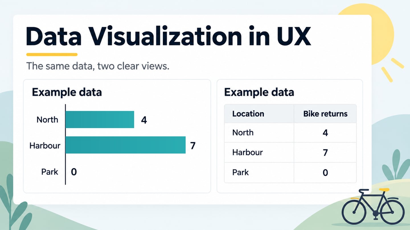
Choose formatting, charts, tables, totals or sparklines according to the question. A chart can reveal a pattern, while a table is useful for exact values. Keep units, missing values and the sample scope visible; a decorative format cannot correct an unsuitable calculation.
Use the Findings in a Design Prototype
After analysis, a Mockitt prototype can make a proposed design response discussable. Arrange screens, labels and interactions around a question suggested by the evidence. Mockitt’s role here is to communicate an interface idea, not to replace Excel formulas, calculate the dataset or automatically import a working analysis.
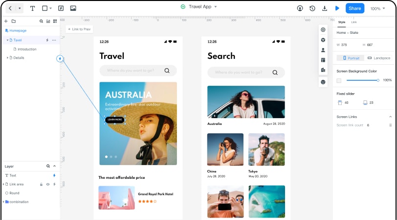
Use reusable elements and a shared preview to explain the proposed change to collaborators. Include the relevant source context and collect feedback on the design decision. The retained travel-app screenshot is a historical interface example, not a demonstration of Excel integration.
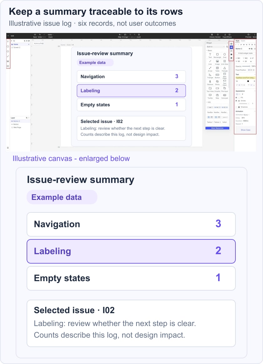
For the illustrative issue log, show a review summary with Navigation 3, Labeling 2 and Empty states 1, then open one labeling issue to discuss a clearer label. Identify the source as Illustrative issue log. The counts establish the composition of this example, not which change will have the greatest impact. Follow up with usability testing when you need evidence about the proposed interface.